Winter by the numbers

 How cold was it this winter?

In today’s era of global warming, much is written about the type of winters we are experiencing. Above average warmth, normal, or colder than usual? This is often given in terms of average temperature for the season: 2 degrees above normal, 2 degrees below normal, etc. I’ve never been satisfied with reference to “average temperature”, because there is so much rolled up into that average. Winter is characterized by the diurnal cycle, the seasonal swing, movements of the jet stream, and so on. It seems to me that a better measure of coldness or warmth is the number of days below or above the long-term historical average, taken day by day. This is a time-weighted view of temperature excursions that adapts better to the expected cycles of the season. So here’s what I have come up with. Comments are welcome.

I found a really nice display of temperatures at a website called WeatherSpark. They use NOAA data obtained at several stations in Vermont and create a visually compelling plot like this, for the station at Caledonia Airport near Lyndonville, in 2022-2023:

There is one gray bar for each day of the season, denoting daily maximum and minimum. A smooth blue curve is the historical daily minimum, where “historical” means the last century. St. Johnsbury, Vermont, has one of the longest well-instrumented stations, covering 1894 to the present. The smooth red curve is the historical daily high, and the shaded bands represent quantiles, apparently. A quick glance tells us that we had deep cold spells in early February and again in late February, not uncommon in the northern hemisphere. We had a few days well below historical average temperature, but these were cold “snaps” lasting only a few days.  The notable warm departure was at Christmas, extending into the first week of January: almost two weeks of freakish global-warming weather.

My method of gauging severity of warmth or cold starts with comparing the gray bar to the blue and red curves. If the whole bar is below the blue curve, we assess it as below-normal temperature; if the whole gray bar is above the red, we have an above-normal day. Anything else is a normal winter day. So, if the daily high never exceeds the historical norm for that day, it gets flagged. Same for when the coldest temperature of the day remains above the red.

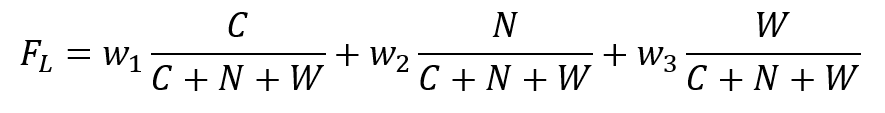
Now count the number of the days over the whole winter season, November to March. (This is the period when we burn the bulk of the propane at my house.) Using C for the number of below-average cold days, W for above-average warm, and N for normal, compute the following:

This quantity F_L is a measure of the departure from normal temperatures, summed over the whole season. It is linear in C and W, hence the subscript L. It ranges from -1 to +1, with zero being a normal winter. If there is an equal number of anomalous warm and cold days, F_L is zero: we assign that year to be normal. This quantity is a reasonable starting point, but it has drawbacks. First of all, the practical range is much smaller than -1 to +1. We’ll never see an entire winter of above-normal warm days (C=N=0, the F_l = +1 condition). Most winters will have roughly 1/2 of the days being normal. In a really warm winter, the remaining 1/2 might be divided up into 40% warm, 10% cold. This yields F_L = +0.3. On the other hand, if there are only a few more warm days than cold days, we shouldn’t be too concerned about it: it’s essentially a normal winter.  So if we have 20 warm days, 6 cold days, and C+N+W = 151, then F_L = 0.093. What we need is a nonlinear function that “stretches” F_L so that the high values are transformed into a really big number, but the small values stay near zero. I think a reasonable nonlinear function is sinh, which also has the nice property that the negative branch is symmetrical with the positive branch. We can write 

F_N = a sinh (bF_L)

and choose some suitable parameters a and b to give a reasonable amount of “stretch”. Somewhat arbitrarily, I chose a = 6, b = 10.

Astute readers will recognize that the quantity F_N has the form of a “artificial neuron” in neural network analysis. The quantity F_L is a dot product between the vector f of fractions of cold, normal, warm days and a weight vector w:

where the weight vector is w = [-1,0,+1].  The (nonlinear) transfer function  is 

Here, though, the transfer function ranges from -∞ to +∞ rather than the customary -1 to +1; in neural networks, the tanh(x) function is typically used rather than sinh(x). But this is suggestive of the fact that, generally speaking, the assessment of seasonal cold/warmth is a problem that lends itself well to machine learning, where one could incorporate many other climatic observations (precipitation, clouds, wind, snow depth, etc.) and where physics-based models may not be terribly useful. The key problem is how to establish a training set of data. A problem for another day.

Returning to the use of the metric F_L, this approach (importing the data, parsing, assigning labels) required about 200 lines of Python code (at least for this Python amateur). So here are the results for St. Johnsbury winters, 1998-2022.

 

Figure 1 Linear metric. Winters in St. Johnsbury, VT, from 1998 to 2022

Figure 2 Non-linear, or sinh, metric for the same data in Fig. 1.

We can see that 2015 (i.e. winter of 2015-16) was an extraordinary warm year. By the count of my method, there were 79 normal days, 10 below normal, and 63 above normal days. Looking at some other compiled state-wide statistics on the web, I am thinking that this winter was about once-per-century warm. The 2001 and 2011 winters were also warm, but reflecting a frequency more like once per 20 years or so. In fact, I have used scaling parameters on the sinh function (a=6, b=10) to achieve F_n values that are in the ball park of these frequency values. The nonlinear scaling also tends to cluster most years at values close to zero, which I think is reasonable.

So what does global warming look like from the standpoint of St. Johnsbury? In the last 25 years, we have had 4 abnormally warm winters, and 4 notably cold winters. This doesn’t sound much like global warming. But the warm bars on the plot are noticeably larger than the cold bars on the plot. So, warming is the trend. I would make the cautionary note, though: global warming doesn’t mean the end of the occasional cold winter. The temperature data analyzed by my method shows that fairly convincingly.

How does my metric for warm/cold winters compare with others widely in use? Here’s a comparison of my F_n with seasonal average temperatures, which I discussed above. I obtained a seasonal average by examining the mid-point of the low and high temperatures for each day, and summing all of them for the whole season. These were compared to the historical record, simply averaged over the whole winter season. I take the difference between these seasonally-based averages, so the units are degrees C.

 

Figure 3 The nonlinear metric (top) compared to simple seasonal averages (bottom).

Overall, the pattern of positive and negative bars is similar. But the seasonal average method tends to exaggerate the cold winters, and suppress the warm winter deviations from zero. So beware of seasonal averages. If anything, they may actually be understating the degree of warming that we are seeing.

What improvements can I make to my method? It would be nice to incorporate the magnitude of the temperature deviation from normal. So a day that is 10 degrees lower than the historical average low would get a larger score than a day that is 2 degrees below historical. The problem, though is coming up with a scheme to “score” the departure from normal. Still pondering that one.